Multivariate Analysis Techniques for Exploring Data

Most problems we deal with have multiple variables. To analyze these variables before they can be used in training a machine learning framework, we need to analytically explore the data. A fast and easy way to do this is bivariate analysis, wherein we simply compare two variables against each other. This can be in the form of simple two-dimensional plots and t-tests.

However, comparing only two variables at a time does not give deep insights into the nature of variables and how they interact with each other. Consider the Curiosity rover recently launched by NASA. It is using laser-induced breakdown spectroscopy (LIBS) to analyze the chemical composition of the rocks in the Gale Crater region of Mars. Now, this data is highly multivariate in nature with over 6000 variables per sample. Imagine plotting two-dimensional graphs to understand the patterns in the data! This is where the need to understand and implement multivariate analysis techniques comes in.

We now look at some of these techniques in detail.

Pairwise plots

Pairwise plots are a great way to look at multi-dimensional data, and at the same time maintain the simplicity of a two-dimensional plot. As shown in the figure below, it allows the analysts to view all combinations of the variables, each in a two-dimensional plot. In this way, they can visualize all the relations and interactions among the variables on one single screen.

Spider Plots

While there are various ways of visualizing multi-dimensional data, spider plots are one of the easiest ways to decipher the meaning of data. From the figure below, we can see how easily we can compare three mobile phones based on attributes such as their speed, screen, camera, memory and apps.

Correlation Analysis

Often, data sets contain variables that are either related to each other or derived from each other. It is important to understand these relations that exist in the data. In statistical terms, correlation can be defined as the degree to which a pair of variables are linearly related. In some cases, it is easy for the analyst to understand that the variables are related, but in most cases, it isn’t. Thus, performing a correlation analysis is very critical while examining any data. Furthermore, feeding data which has variables correlated to one another is not a good statistical practice, since we are providing multiple weightage to the same type of data. To prevent such issues, correlation analysis is a must.

Cluster Analysis

In many business scenarios, the data belongs to different types of entities; and fitting all of them into a single model might not be the best thing to do. For example, in a bank dataset, the customers might belong to multiple income groups which leads to different spending behaviors. If we use the data having all these customers into a single model, we would be comparing apples to oranges. In that regard, clustering provides analysts a good way to segment their data and therefore avoid this problem. Clustering also allows us to visually understand and therefore compare the different attributes of the segments formed.

K-means clustering is a well-renowned approach used by a lot of data analysts and scientists. This separates the data points into clusters such that the inter-cluster distances are maximized. What this means is that each point in a particular cluster is similar to every other point in that cluster; and, points in a particular cluster are very different from every point in any other cluster. Other popular approaches for clustering include the hierarchical clustering algorithm, the DBSCAN algorithm, Partitioning Around Medoids (PAM) algorithm, etc.

MANOVA (Multivariate Analysis of Variance)

This technique is best suited for use when we have multiple categorical independent variables; and two or more metric dependent variables. While the simple ANOVA (Analysis of Variance) examines the difference between groups by using t-tests for two means and F-test otherwise, MANOVA assesses the relationship between the set of dependent features across a set of groups. For example, this technique is suitable when we want to compare two or more dishes in a restaurant against each other, in terms of the level of spiciness, the time taken to cook and value for money, etc.

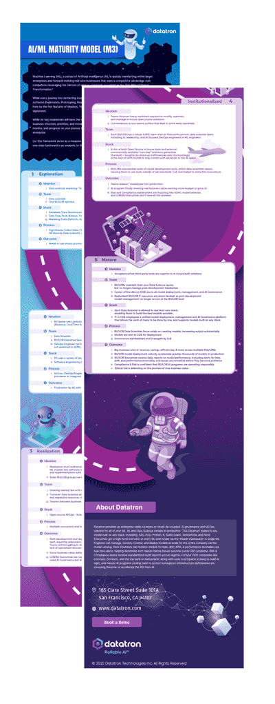
Infographic

MLOps Maturity Model [M3]

In this Infographic, you’ll learn:

The FIVE stages of maturity in Machine Learning Operations, i.e., MLOps
Why DevOps is not the same for ML as it is for software, and why MLOps is needed
The ideal teams, stacks, and features to look for to reach Maturity in your ML program

Learn why some companies succeed, while others struggle in AI/ML by seeing the signatures of success across Ideation, Team, Stack, Process, & Outcome in this informative (Hi-res) Infographic.

Infographic: MLOps Maturity Model [M3]

Principal Component Analysis and Factor Analysis

Although machine learning is a game of predicting the result given multiple predictors, there can be times when the number of these predictors is too large. Not only is such a data set difficult to analyze, but the models formed using this are susceptible to overfitting. Therefore, it makes sense to have the number of these variables reduced. Principal component analysis (PCA) and Factor analysis are two of the common techniques used to perform such a dimension reduction.

PCA reduces the existing number of variables, such that the new set of reduced variables capture most of the total variance present in the existing set of variables. Many times, we usually have only two or three features in this new set of features. What this allows us is to visualize all of the initial information in 2-D or 3-D plots, and thus aid in exploratory data analysis. Furthermore, these new features are a combination of the initial features which helps us understand the variables which are important.

Therefore, PCA is such a powerful tool for analysts since they now have a much smaller feature set to deal with, and at the same time having preserved most of the information which was initially present. While PCA extracts factors based on the total variance, the Factor Analysis Method extracts factors based on the variance shared by the factors. By providing the factors based on the variance they share, Factor Analysis enables data scientists to examine the underlying trends in the data.

Discriminant Analysis

This is used to classify two or more groups of data and differentiate among them. The best use of this technique is when the dependent variable is categorical and the independent variables are metric. Discriminant analysis develops discriminant functions, which are linear combinations of the independent variables. These functions help in distinguishing between the categories in the dependent variable. They enable the analyst to quickly look at whether the differences between the groups are significant. For example, it can help distinguish between heavy, moderate and low spenders depending upon customer attributes like age, gender, income, etc.

Conjoint Analysis

Conjoint analysis, also known as trade-off analysis, is a very important tool used in marketing. It helps in identifying whether customers like different attributes of a product/service or not. It also helps in identifying the preference of customers to a particular feature over others. Smartphone companies often use this analysis to understand the combination of attributes such as features, color, price, dimensions, etc. that customers favor. They use the results of such analyses in their strategies to drive profitability.

Multiple Regression Analysis

Having looked at the multiple ways of exploring and making sense of data in the data processing stage, we now shift gears to regression analysis. Regression is one of the simplest yet powerful techniques to analyze data. While simple regression maps one variable as a function of the other, multiple regression maps one variable (called the dependent variable) as a function of several other variables (called independent variables or predictors). Doing such an analysis gives us an equation of the form:

where, α is the intercept, βi are the coefficients, y is the dependent variable, and xi are the predictors. We can read this equation as: For every unit increase in xi, the value of y increases by βi units. Thus, such analysis allows us to observe how the behavior of the dependent variable changes with respect to other variables. This helps us understand the interactions among variables, and create a visual map of how changes in the predictors can lead to change in the target variable.

Summing up, we have handpicked the top multivariate analysis techniques used in the data science industry. It is no surprise that data analysis and data processing comprise the majority of the work that goes into the development of a machine learning model. In that regard, the techniques explained in this article are a go-to reference for all data analysts, engineers and scientists out there. To further understand the management of multivariate models through A/B testing for live inference as well as batch tasks, please visit Datatron

Infographic

MLOps Maturity Model [M3]

In this Infographic, you’ll learn:

The FIVE stages of maturity in Machine Learning Operations, i.e., MLOps
Why DevOps is not the same for ML as it is for software, and why MLOps is needed
The ideal teams, stacks, and features to look for to reach Maturity in your ML program

Learn why some companies succeed, while others struggle in AI/ML by seeing the signatures of success across Ideation, Team, Stack, Process, & Outcome in this informative (Hi-res) Infographic.

Datatron Blog

Blog Category

Search